A Python toolkit for producing publication-quality microeconomics diagrams. Define utility functions declaratively, solve for consumer equilibria, and export figures as PNG, PDF, SVG, or pure TikZ, all in a few lines of code.

Installation

pip install utility-viz

Requires Python 3.10 or later. The current release is a pre-release (2.0.0b2); while no stable 2.x exists, pip install utility-viz picks it up. Once a stable release is published alongside it, use pip install --pre utility-viz to opt in to pre-releases.

Upgrading from econ-viz 1.x? See Migrating from econ-viz.

Quick Start

from utility_viz import Canvas, Fill, Marker, levels, solve, themes
from utility_viz.models import CobbDouglas

model = CobbDouglas(alpha=0.5, beta=0.5)
eq = solve(model, px=2.0, py=3.0, income=30.0)
lvls = levels.around(eq.utility, n=5)

cvs = Canvas(
    x_max=20,
    y_max=15,
    x_label="x",
    y_label="y",
    title="Cobb-Douglas  $x^{0.5} y^{0.5}$",
    theme=themes.monochrome,  # black/grey only, lines told apart by style
    dpi=120,
)
cvs.add_utility(model, levels=lvls)
cvs.add_budget(2.0, 3.0, 30.0, fill=Fill(color="lightgrey", opacity=0.5))
cvs.add_equilibrium(eq, show_ray=True, marker=Marker(size=8))
cvs.save("cobb_douglas_eq.png")

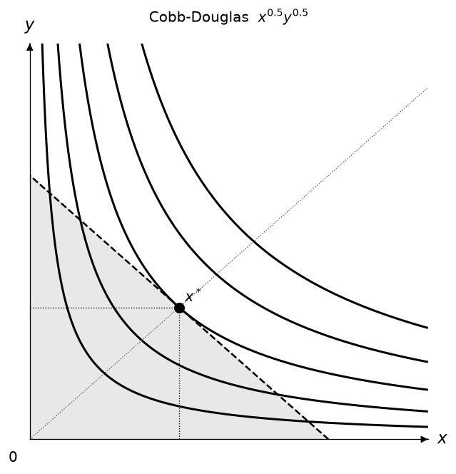
Without theme= the default colour-blind-friendly palette is used.

TikZ export writes a standalone LaTeX document with only TikZ drawing commands:

cvs.save("cobb_douglas.tex", tikz_scale=0.0125)

tikz_scale is centimetres per Matplotlib pixel (at 100 dpi); the default, 0.0125, maps a 6 inch wide Matplotlib figure to 7.5 cm.

Notebook

The project ships with an interactive playground notebook:

notebook/econ-viz Playground.ipynb

The file keeps its historical name. Download it and open it in Jupyter, VS Code, or Colab. The first code cell installs utility-viz[all] (pinned to 2.0.0b2) from PyPI for fresh runtimes.

Highlights

• Built-in models (also listed by utility-viz models): Cobb-Douglas, Leontief, Perfect Substitutes, CES, Satiation, Quasi-Linear, Stone-Geary, and Translog
• Built-in themes, including a black-and-white themes.monochrome for print
• Solver support for interior, kink, boundary, and corner solutions
• Closed-form demand helpers with solution_tex(...)
• Comparative tools including comparative_statics(...) and slutsky_matrix(...)
• Multi-panel Figure layouts, PricePath / IncomePath, and linked DemandDiagram
• CLI support for plotting and closed-form demand output
• Color-blind-friendly default palette (themes.COLORBLIND_CYCLE_RGB) sourced from thriveth/8560036, with related citation at DOI:10.1080/00220485.1996.10844911

Additional Tools

Axis labels can be placed around their arrowheads, and each axis can use its own arrowhead style and line style (solid, dashed, dotted, or dashdot):

from utility_viz import ArrowStyle, Canvas, LabelPosition, LineStyle

canvas = Canvas(
    x_label_pos=LabelPosition.TOP,
    y_label_pos=LabelPosition.RIGHT,
    x_arrow_style=ArrowStyle.SIMPLE,
    y_arrow_style=ArrowStyle.WEDGE,
    x_line_style=LineStyle.DASHED,
)

Every line can be restyled with a Stroke: width, line style, colour, and an arrowhead at its end. Fields you leave out keep the theme default (see the *_stroke defaults on Theme, such as theme.budget_stroke):

from utility_viz import ArrowStyle, Stroke

canvas = Canvas(axis_stroke=Stroke(width=1.4, arrow=ArrowStyle.SIMPLE))
canvas.add_budget(2, 3, 30, stroke=Stroke(width=3, style="dashed"))
canvas.add_equilibrium(eq, drop_stroke=Stroke(style="dashdot"))
canvas.add_ray(0.5, stroke=Stroke(arrow=ArrowStyle.TRIANGLE))

add_utility, add_path, add_decomposition, DemandDiagram, and EdgeworthBox take one *_stroke argument per kind of line they draw. Stroke is the preferred way to style lines; the separate color, linewidth, and linestyle arguments still work as shorthand and draw the same thing.

Point markers work the same way with Marker (colour, size, and shape); fields you leave out keep the theme default, such as theme.eq_marker:

from utility_viz import Marker

canvas.add_equilibrium(eq, marker=Marker(shape="s", size=8))
canvas.add_point(12, 2, label="A", marker=Marker(color="black", shape="D"))
canvas.add_decomposition(dec, point_marker=Marker(shape="^"))

Point labels take a Label (text, position, offset, colour, size, and visibility) wherever a plain string worked. A label follows its point's Marker colour unless it sets its own:

from utility_viz import Label

canvas.add_equilibrium(eq, label=Label(position="bottom-left", offset=8))
canvas.add_point(12, 2, label=Label(text="A", position="left", fontsize=14))
canvas.add_utility(u, levels=3, ic_label=Label(text="U={:.1f}", position="top"))
canvas.add_decomposition(dec, point_label=Label(visible=False))  # hide A, B, C

The same Label styles every other piece of text: axis labels, the origin 0, titles, effect labels, and the Edgeworth box's good names and origins:

from utility_viz import Axis, Canvas, Effect, Label

canvas = Canvas(
    title=Label(text="Hicks decomposition", fontsize=13),
    x_axis=Axis(label=Label(text="x_1", fontsize=16)),
    origin_label=Label(visible=False),
)
canvas.add_decomposition(dec, substitution=Effect(label=Label(text="SE", fontsize=12)))

Shade the budget set with fill=True, or pass a Fill for a colour and opacity of its own (default theme.budget_fill, coloured like the line):

from utility_viz import Fill

canvas.add_budget(2, 3, 30, color="black", fill=Fill(color="lightgrey", opacity=0.4))

Every style object takes an opacity from 0 to 1, for example to show the original budget line faintly:

from utility_viz import Effect, Legend, Stroke

canvas.add_budget(2, 3, 30, stroke=Stroke(opacity=0.35))
canvas.add_decomposition(dec, income=Effect(opacity=0.5), legend=Legend(opacity=0.8))

Each axis's label, label position, and stroke fit in one Axis, accepted by Canvas, Figure, DemandDiagram, and EdgeworthBox. x_label, x_label_pos, and x_axis_stroke stay as shorthand; an Axis field wins when both are set:

from utility_viz import Axis, Stroke

canvas = Canvas(
    x_axis=Axis(label="x_1", label_position="bottom", stroke=Stroke(width=1.2)),
    y_axis=Axis(label="x_2"),
)

Legends go where they cover the least of the diagram by default, moving outside the plot area when every corner is taken. Pass a Legend to choose an inside corner ("upper left", …) or a side outside ("top", "bottom", "left", "right"), or to change its font size, frame, and columns:

from utility_viz import Legend

canvas.add_decomposition(dec, legend=Legend(position="bottom"))
canvas.show_legend(legend=Legend(position="upper left", fontsize=10))

Set a font for one canvas or a whole multi-panel figure without touching Matplotlib's global settings. Pass a family name, a generic family such as "serif", or a fallback list:

from utility_viz import Figure, Layout

canvas = Canvas(font=["Times New Roman", "serif"], math_font="stix")
figure = Figure(Layout.SIDE_BY_SIDE, font="serif", math_font="stix")

font applies to titles, axis labels, annotations, curve labels, and legends. Math text, including the default axis labels, uses math_font: "stix" (Times-like), "cm" (Computer Modern), "dejavuserif", "dejavusans", or "stixsans". An unavailable font raises InvalidParameterError. TikZ output uses the LaTeX document's fonts, so only generic families are mapped (serif → \rmfamily, monospace → \ttfamily).

Closed-form Marshallian demand in TeX:

from utility_viz import solution_tex
from utility_viz.models import CobbDouglas

tex = solution_tex(CobbDouglas(alpha=0.4, beta=0.6))

Slutsky matrix:

from utility_viz import slutsky_matrix
from utility_viz.models import CobbDouglas

S = slutsky_matrix(CobbDouglas(alpha=0.4, beta=0.6), px=2.0, py=3.0, income=60.0)
# S.s_xx, S.s_xy, S.s_yx, S.s_yy

Settings file

Keep your style in a utility-viz.toml and load it once. Section names match Theme properties ([stroke.budget] is theme.budget_stroke), fields match the style objects, and anything left out keeps the default:

[color]
ic = "#2E86AB"

[stroke.budget]
width = 1.5

[label.point]
fontsize = 12

[legend]
position = "bottom"

from utility_viz import Config

Config.load("utility-viz.toml").use()  # diagrams created from now on use it

utility-viz init writes a commented template, and utility-viz plot --config utility-viz.toml ... uses the same file. Arguments passed to a method still win over the file.

CLI

utility-viz --version
utility-viz help
utility-viz models
utility-viz solve-tex --model cobb-douglas --symbolic-params

Plotting example:

utility-viz plot --model cobb-douglas --alpha 0.5 --beta 0.5 \
              --px 2 --py 3 --income 30 \
              --fill --show-ray \
              --output cobb_douglas.png

Migrating from econ-viz

econ-viz was renamed to utility-viz in 2.0.0.

	1.x	2.x
Distribution	pip install econ-viz	pip install utility-viz
Import	import econ_viz	import utility_viz
CLI	econ-viz	utility-viz
Config file	econ-viz.toml	utility-viz.toml (section names unchanged)

Which package to install. utility-viz ships only utility_viz and the utility-viz command: it has no econ_viz package and no econ-viz command. econ-viz 2.x (same version number) is a thin compatibility distribution: pip install econ-viz installs utility-viz of the same version plus the econ_viz package and the econ-viz command, which warn that they are deprecated. Upgrading an existing 1.x installation with pip install --upgrade econ-viz therefore keeps working and moves you onto 2.x. Pre-releases need --pre (for example pip install --pre --upgrade econ-viz). Switch to pip install utility-viz when you are ready to drop the compatibility layer.

Compatibility layer. Throughout 2.x the econ-viz distribution provides an econ_viz package and an econ-viz command so documented 1.x code keeps working:

• import econ_viz emits one deprecation warning per process.
• from econ_viz import ... and the documented sub-modules (econ_viz.models, econ_viz.optimizer, econ_viz.themes, ...) resolve to their utility_viz equivalents. Names that did not change are the very same objects.
• Constructing econ_viz.Canvas, econ_viz.Figure or econ_viz.animation.Animator, or accessing econ_viz.Layout, emits a utility_viz.UtilityVizDeprecationWarning (a FutureWarning) stating "deprecated since 2.0.0, removed in 3.0.0" and the replacement. Figure, Layout and Animator map to their current 2.x equivalents; their declarative replacements (CanvasGrid, Animation) are planned and named in the message as such.
• Config lookup: explicit path, then utility-viz.toml, then legacy econ-viz.toml (with a warning), then defaults. If both files exist the new one wins and the legacy one is ignored with a warning. Config.load() with no argument follows the file order and raises if neither file exists (as in 1.x); Config.discover() falls back to defaults; Config.load("file.toml") reads exactly that file. utility-viz plot applies the same lookup in the current directory when --config is not given.
• The econ-viz command prints a deprecation warning and forwards to utility-viz.
• utility-viz init --migrate writes utility-viz.toml from econ-viz.toml and keeps the old file.

Removal boundary (3.0.0). The econ_viz package, the econ-viz command and econ-viz.toml lookup are removed in 3.0.0, not 2.0.0. Only the documented 1.x public API is covered; undocumented deep module paths (for example econ_viz.canvas.renderers.*) resolve on a best-effort basis and may disappear at any time. Internal utility_viz.core.* modules are advanced APIs and not part of the compatibility contract.

Ecosystem

utility-viz is part of the EconViz family of packages:

• mosaickit (PyPI): domain-neutral scenes and rendering, which utility-viz renders through.
• bezierkit (PyPI): Bezier curves, used by utility-viz for curves and TikZ output.
• principle-viz (PyPI): the sibling package for principles-of-economics diagrams.

Documentation

Full documentation lives at econ-viz.org. Source and issues: github.com/EconViz/utility-viz.

License

MIT © Pin Yue Sung